Targeted elevation mapping with grayscale contrast using R
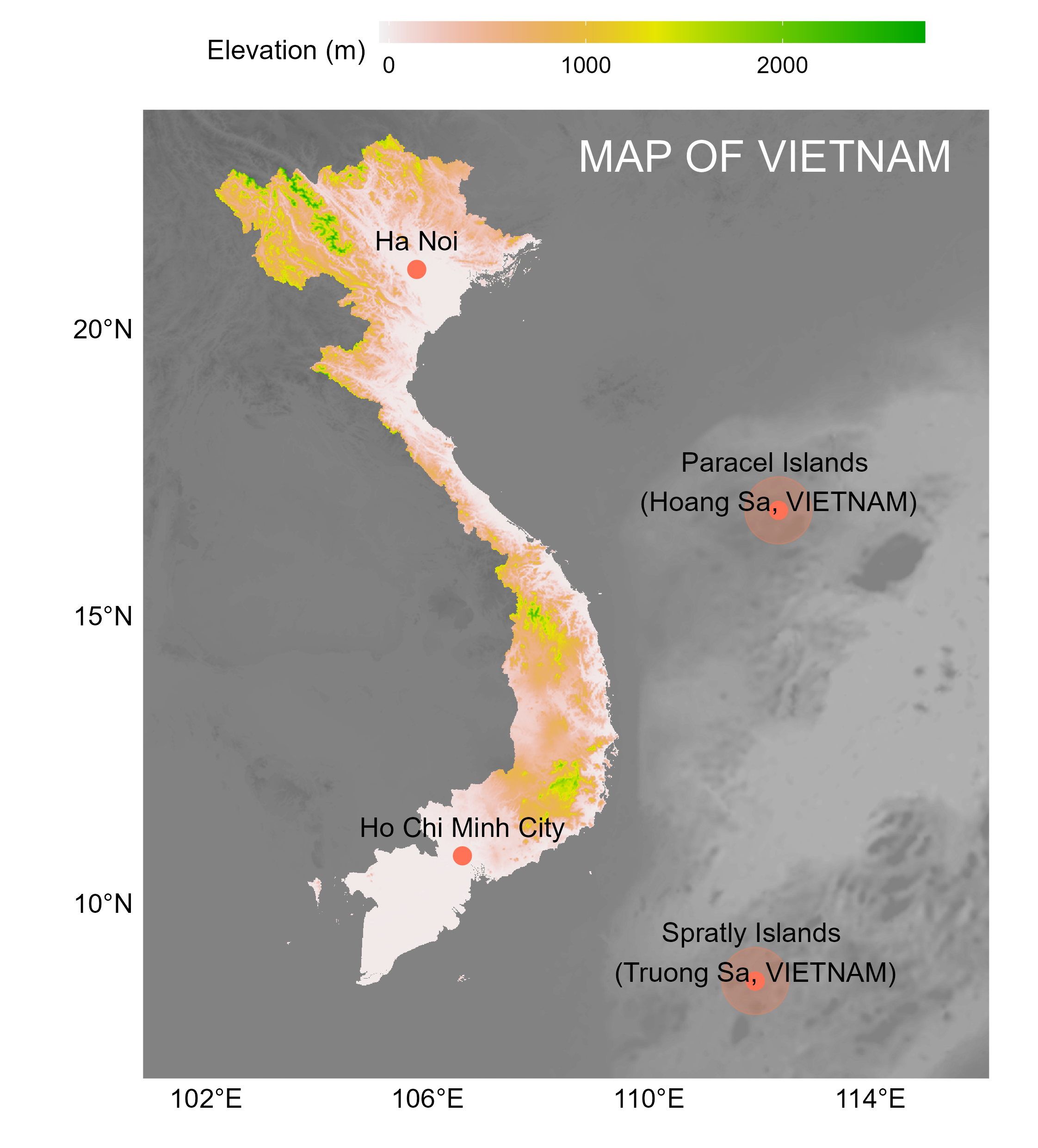
This blog post serves as a step-by-step guide to generating stunning elevation maps in R. The elevation map highlights a specific area of interest in vibrant color against a grayscale background of neighboring landscapes. Using Vietnam as featured example, this post will showcase the power of R in visualizing elevation data.
The complete code for this visualization is available on Github.
library(tidyverse)
library(here)
library(elevatr)
library(raster)
library(sf)
library(scales)
Step 1: Specify the boundaries of the map drawing rectangle
Set the plot boundaries using coordinate data.
The coordinate can be obtained from several websites, for example, bboxfinder.com.
bounds_data <- data.frame(x = c(100.854490, 116.147458), # longitude
                          y = c(6.945000, 23.812699) # latitude
                          )
Step 2: Get the elevation of background raster
Note: Change the zoom level if getting Error: cannot allocate vector of size XXX Mb.
# set projection
proj <- "+proj=longlat +ellps=WGS84 +datum=WGS84 +no_defs"

# get elevation raster
background_raster <- elevatr::get_elev_raster(locations = bounds_data,
                                              # projection
                                              prj = proj,
                                              # set the zoom level to return; the value ranges from 1 to 14
                                              z = 6,
                                              # determine clipping of returned DEM
                                              clip = "locations")
Step 3: Read the polygonal file to outline the boundary of Vietnam
The polygonal data can be downloaded from several websites, for example, diva-gis.
# corresponding file format: SHAPEFILE (.shp)
terrain_extent <- sf::st_read(here::here("data/VNM_gis/VNM_adm0.shp"))
Step 4: Retain the boundary of Vietnam to display the terrain raster
terrain_raster <- raster::mask(background_raster, terrain_extent)Step 5: Modify RasterLayer data to be compatible with ggplot2
- Convert the RasterLayer into a data.frame format
- Adjust the value range of the layer (elevation)
# background part
names(background_raster) <- "layer"
background_raster_df <- as.data.frame(background_raster, xy = TRUE) %>%
                                mutate(alpha = rescale(layer, to = c(0.25, 0.75)))

# terrain part
names(terrain_raster) <- "layer"
terrain_raster_df <- as.data.frame(terrain_raster, xy = TRUE) %>%
                                mutate(alpha = ifelse(is.na(layer), 0, 1))
Step 6: Create the map using ‘ggplot2’
# set scale value to control size of text, point, legend, etc. to fit figure size
scale_value <- 2

# initial ggplot
gmap <- ggplot() +
        # plot background layer
        geom_raster(data = background_raster_df,
                    aes(x = x, y = y, alpha = alpha)) +
        # plot terrain layer
        geom_raster(data = terrain_raster_df,
                    aes(x = x, y = y, fill = layer, alpha = alpha)) +
        scale_fill_gradientn(colours = terrain.colors(100, rev = TRUE),
                             # set the legend title for elevation using the 'name' parameter
                             name = "Elevation (m)") +
        # project this plot as a map rather than a standard figure
        coord_quickmap() +
        # modify axis titles
        labs(x = "", y = "") +
        # define axes limits
        # use `expand` parameter to remove the gaps between the rectangular map and axes
        scale_x_continuous(limits = c(100.854490, 116.147458), # longitude
                           expand = c(0, 0),
                           breaks = c(102, 106, 110, 114),
                           labels = c("102\u00B0E",
                                      "106\u00B0E",
                                      "110\u00B0E",
                                      "114\u00B0E")) +
        scale_y_continuous(limits = c(6.945000, 23.812699), # latitude
                           expand = c(0, 0),
                           breaks = c(10, 15, 20),
                           labels = c("10\u00B0N",
                                      "15\u00B0N",
                                      "20\u00B0N")) +
        # remove legend of alpha
        scale_alpha(guide = "none") +
        # modify theme
        theme_minimal() +
        theme(panel.grid = element_blank(),
              panel.background = element_blank(),
              axis.text = element_text(size = 7 * scale_value,
                                       color = "black"),
              legend.position = "top",
              legend.key.width = unit(1 * scale_value, "cm"),
              legend.key.height = unit(0.2 * scale_value, "cm"),
              legend.text = element_text(size = 6 * scale_value),
              legend.title = element_text(size = 7 * scale_value))
Step 7: Incorporate cities and islands into the map
Generate a dataframe containing coordinate data and site names.
site_df <- data.frame(site_name = c("Ha Noi",
                                    "Ho Chi Minh City",
                                    "Paracel Islands \n(Hoang Sa, VIETNAM)",
                                    "Spratly Islands \n(Truong Sa, VIETNAM)"),
                      site_latitude = c(21.028511, 10.823020, 16.83517, 8.64464),
                      site_longitude = c(105.804817, 106.629650, 112.33873, 111.91969))
Incorporate cities and islands into the map using ggplot2
gmap <- gmap +
        # add the areas of islands as large circles on the map
        geom_point(data = site_df %>% filter(str_detect(site_name, "Islands")),
                   mapping = aes(x = site_longitude,
                                 y = site_latitude),
                   size = 8 * scale_value,
                   color = "coral",
                   alpha = 0.3) +
        # add the cities and primary islands as points
        geom_point(mapping = aes(x = site_longitude,
                                 y = site_latitude),
                   data = site_df,
                   size = 2 * scale_value,
                   colour = "coral1") +
        # add names of cities and islands as text labels
        geom_text(mapping = aes(x = site_longitude,
                                y = site_latitude + 0.5,
                                label = site_name),
                  data = site_df,
                  size = 2.5 * scale_value)
Step 8: Add the map title
gmap <- gmap +
        geom_text(mapping = aes(x = 112.1, y = 23, label = "MAP OF VIETNAM"),
                  size = 4 * scale_value,
                  color = "white")
References
- Using R for Everything: 使用 ggplot2 绘制 RasterLayer 地图 by Chen Han
- Elevation data in R by Ivan Lizarazo